A Tutorial for `dsdp`

Satoshi Kakihara¹

Takashi Tsuchiya²

November 11th, 2022

Abstract

This vignette is a tutorial for a R package dsdp, a probability density estimation package using a maximum likelihood method. A model of interest in this package is a family of exponential distributions as base functions, with polynomial correction terms. To find an optimal model, we adopt a grid search for parameters of base functions and degrees of polynomials, together with semidefinite programming for coefficients of polynomials, and then model selection is done by Akaike Information Criterion. We first give a quick overview of the package, and then move on to a tutorial.

Overview

The main task of the package dsdp is to estimate probability density functions from a data set using a maximum likelihood method. The models of density functions in use are familiar Gaussian or exponential distributions with polynomial correction terms. We call Gaussian distribution with a polynomial Gaussian-based model and an exponential distribution with a polynomial Exponential-based model, respectively. dsdp seeks parameters of Gaussian or exponential distributions together with degrees of polynomials using a grid search, and coefficients of polynomials using a variant of semidefinite programming(SDP) problems. Detailed discussions of SDP problem formulations and this type of SDP problems are found in other vignettes.

The outline of estimation procedure is as follows.

1. Create Gaussian-based or Exponential-based model from a data set.
2. Explore a data set by checking the statistics and the histogram
3. Provide a set of parameters of Gaussian or exponential distributions and degrees of polynomials.
4. Estimate the coefficients of the polynomials for a set of parameters and then check the results by comparing Akaike Information Criterion(AIC) and plotting density functions.
5. Refine the parameters and repeat 3-4 until a sufficient estimate is obtained.

We will see each process step by step in the next section. Before we move on, please install and import the package if you haven’t yet. Installation is done by

## Install from CRAN
install.packages("dsdp")

Importing the package is done by

## Import dsdp
library(dsdp)

This package requires ggplot2 for displaying histograms and density functions. ggplot2 is a part of tidyverse, a de facto standard for data wrangling in R. Our plot method returns ggplot2 objects, so if you plan to add the title or change the labels in the graphs, it is better to import ggplot2 too.

## Import ggplot2 if necessary.
library(ggplot2)

A Tutorial

In this section, we will see estimation procedures in Gaussian-based model and Exponential-based model in details. Essentially, they are same in computations, yet there are subtle differences in practice.

Gaussian-based Model

The density function of Gaussian-based model is \[ p(x; \boldsymbol{\alpha}) \cdot N(x; \mu, \sigma^2), \] where \(p(x; \boldsymbol{\alpha})\) is a polynomial with a coefficient vector \(\boldsymbol{\alpha}\), and \(N(x; \mu, \sigma^2)\) is Gaussian distribution with mean \(\mu\) and variance \(\sigma^2\): \[ N(x;\mu, \sigma^2) := \frac{1}{\sigma \sqrt{2\pi}} \exp\left(-\frac{(x-\mu)^2}{2\sigma^2}\right). \]

The aim of estimation is to find a good set of parameters: \(\boldsymbol{\alpha}\), \(\mu\), and \(\sigma\). To this end, we first provide a coarse set of parameters of base functions, namely, \(\mu\) and \(\sigma\), along with degrees of polynomials, and then compute the coefficients of polynomials \(\boldsymbol{\alpha}\), to get a rough idea of the model. And subsequently, refine the set of parameters and repeat above process until sufficient estimate is obtained.

A Creation of a model

We first create Gaussian-based model from a data set. The name of R’s S3 class for Gaussian-based model is gaussmodel, and we refer to the method of gaussmodel as method.gaussmodel, for example, summmary.gaussmodel, plot.gaussmodel, estimate.gaussmodel, func.gaussmodel.

There are two scenarios for model creations. One is to create a model from only a data set, and the other is to create a model from a data set and its corresponding frequency data. Let’s see model creations in examples.

In the first case, we use a data set mix2gauss$n200, which contains 200 realizations of bimodal mixed Gaussian distributions, to create R’s S3 class gaussmodel object gm1.

## Create gaussmodel object from a data set mix2gauss$n200
gm1 <- gaussmodel(data=mix2gauss$n200)

The object gm1, an instance of a S3 class gaussmodel, contains the data and parameters to be estimated.

Similarly, in the second case, we use mix2gaussHist$n200p for data points and mix2gaussHist$n200f for their corresponding frequencies, to create gaussmodel object gm2.

## Create gaussmodel object from a data set mix2gaussHist$n200p and 
## its frequencies mix2gaussHist$n200f
gm2 <- gaussmodel(mix2gaussHist$n200p, mix2gaussHist$n200f)

Exploring a data set

A summary of gm1 is displayed:

## Display the summary of a data set
summary(gm1)

##   SUMMARY
## Name: mix2gauss$n200 
## The number of Data:  200 
## Mean   Std.
## 0.4503117 1.022398 
## Quantile:
##         0%        25%        50%        75%       100% 
## -2.1092675 -0.2774186  0.7110494  1.2108179  2.0967254 
## Quantile of Scaled Data:
##         0%        25%        50%        75%       100% 
## -2.5035068 -0.7117881  0.2550257  0.7438459  1.6103458

As a name suggests, summary.gaussmodel shows the basic statistics of a data set. It prints out the quantiles of standardized data as well as original data. Here standardization means rescaling of data so as to have a mean 0 and a standard deviation 1.

The histogram of the data is displayed:

## Draw a histogram of the data set
plot(gm1)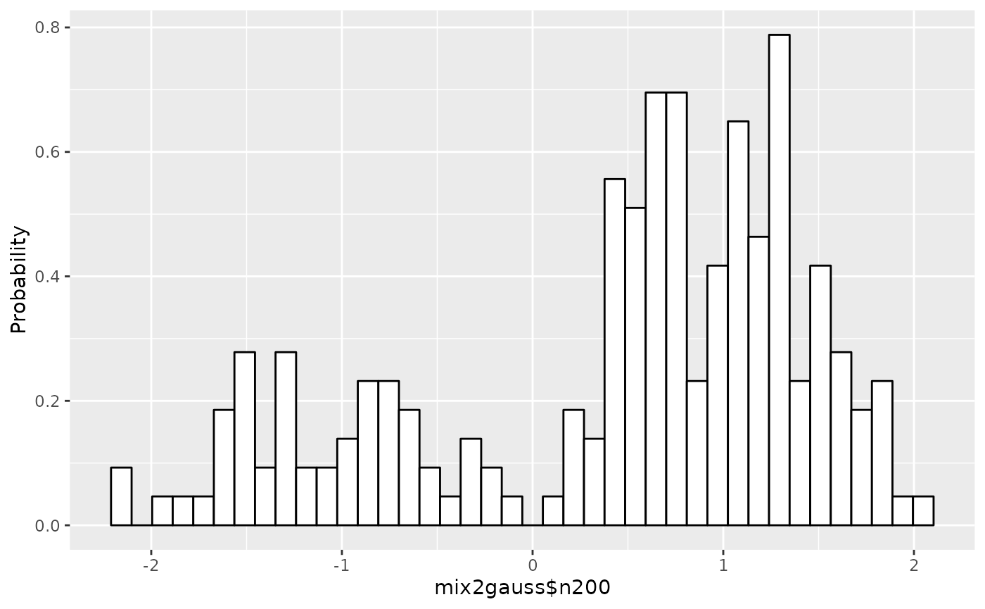

plot.gaussmodel can plot scaled data as well as original data by setting scaling=TRUE.

Providing the set of parameters

Before estimation, we need to provide a set of parameters, means, standard deviations, and degrees of polynomials, to compute the coefficients of polynomials. ````

## A vector of degrees of polynomials
deglist <- c(2, 4, 6)
## A vector of means in Gaussian distributions
mulist <- c(-0.5, 0, 0.5)
## A vector of standard deviations in Gaussian distributions
sdlist <- c(0.75, 1.0, 1.25)

A vector deglist indicates degrees of polynomials, in this case 2, 4, 6. In Gaussian-based model, a positive even integer up to around 20 is okay. Note that large degrees can cause numerical difficulty. mulist is a vector of means of Gaussian distribution, and sdlist is a vector of standard deviations of Gaussian distribution, so the element of sdlist should be positive.

Note that we set these data for estimation of scaled data, as we will mention later.

Estimation

Providing these parameter sets, we are now ready to estimate the model.

## Do estimation
## Output messages are suppressed for brevity
gm1 <- estimate(gm1, deglist=deglist, mulist=mulist, sdlist=sdlist, scaling=TRUE)

The computation of the coefficients of the polynomials is done for all of the combinations of the parameter sets deglist, mulist, and sdlist, 9 cases in this example. By setting scaling=TRUE, estimation is done for scaled data, not for original data, as mentioned before. The result is sorted according to Akaike information criterion(AIC). AIC is widely used criterion for model selection so as to avoid overfitting by penalizing the number of free parameters.

Let’s see the result of estimation.

## Show the summary of results up to 5
summary(gm1, nmax=5, estonly=TRUE)

##   ESTIMATION
## Name: mix2gauss$n200 
##   deg         mu1      sig1   mu  sig      aic     accuracy
## 1   6  0.96151051 0.7667982  0.5 0.75 149.9553 7.159002e-08
## 2   6  0.45031175 0.7667982  0.0 0.75 150.2469 7.345730e-08
## 3   4  0.45031175 0.7667982  0.0 0.75 150.9287 5.479310e-08
## 4   6 -0.06088702 0.7667982 -0.5 0.75 152.5820 7.559624e-08
## 5   4 -0.06088702 0.7667982 -0.5 0.75 157.0336 5.499543e-08

(nmax=5 limits top 5 estimates, and estonly=TRUE suppresses the basic statistics.)

The columns of deg, mu1 and sig1 indicate the degree of polynomials, mean, and standard deviation, respectively. And the columns of mu and sig indicate the scaled mean and standard deviation, respectively.

The column of aic indicates AIC and that of accuracy does the accuracy of the underlying SDP solver, whose value around \(1.0^{-7}\) is sufficient for estimation under IEEE 754
double precision. If sufficient accuracy is not achieved because of numerical difficulty, set recompute=TRUE and stepsize=c(0.4, 0.2), for example, and try recomputation.

## This is demonstration for recomputation
## Not Executed
gm1 <- estimate(gm1, deglist=deglist, mulist=mulist, sdlist=sdlist, scaling=TRUE,
          recompute=TRUE, stepsize=c(0.4, 0.2))

The flag stepsize indicates the vector of step sizes of the underlying SDP solver. The smaller the values are, the better the chances of successful estimation, but the slower the computation is. The default value of stepsize is c(0.5, 0.3), which is enough in many cases. We will not discuss the implementation details here, but if the user sets stepsize by oneself, the user should set the values smaller than default values and the length of two is enough.

The numbers 1,2,3,… in the leftmost column indicate the indices of estimates ordered by AIC. First row is the best estimate, second row is the second best, so on, and these numbers can be used in plot.gaussmodel or func.gaussmodel to designate the estimates to be plotted or evaluated, respectively.

To see the graphs of estimated densities along with the histogram, simply type:

plot(gm1)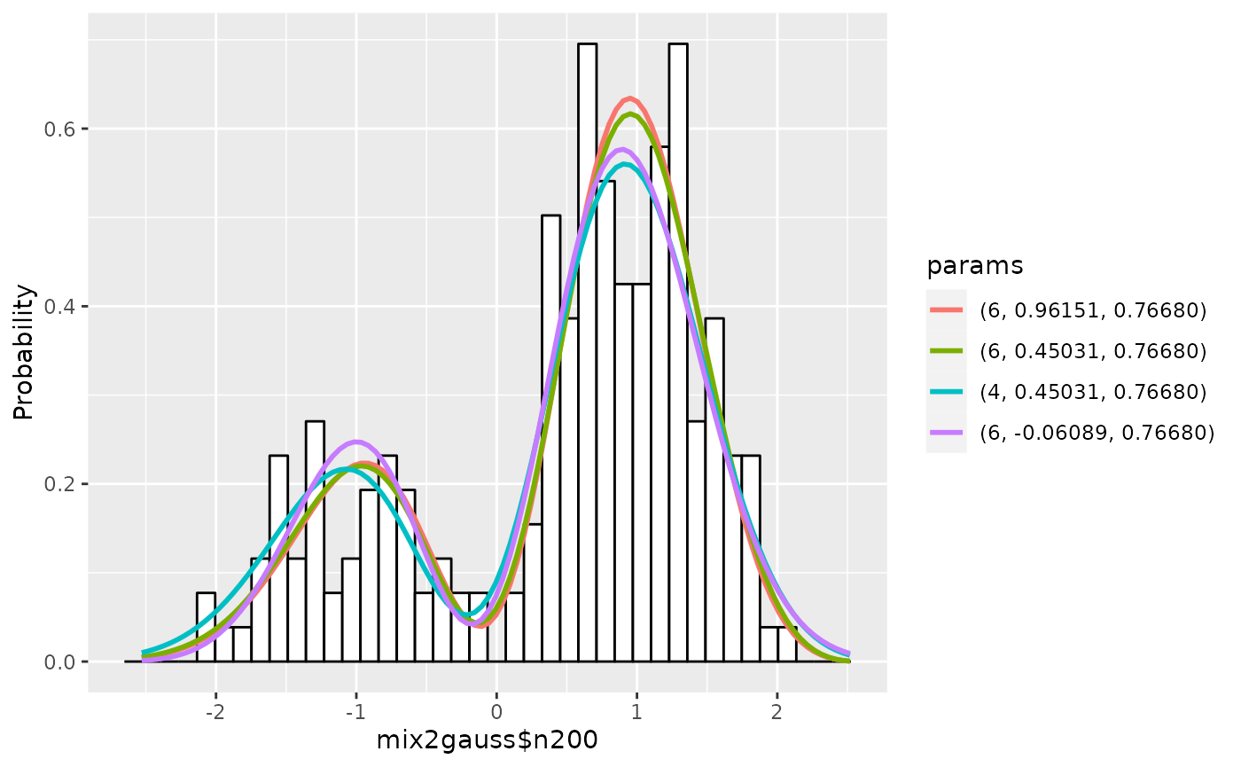

By default, plot.gaussmodel plots up to best 4 estimated density functions. In the legend, the color of graphs are displayed in increasing order of AIC. For example, in this graph, the estimation with the degree 6, mean 0.96151, standard deviation 0.76680 is the best one.

By setting scaling=TRUE, it can plot a scaled data, like scaled graphs.

plot(gm1, scaling=TRUE)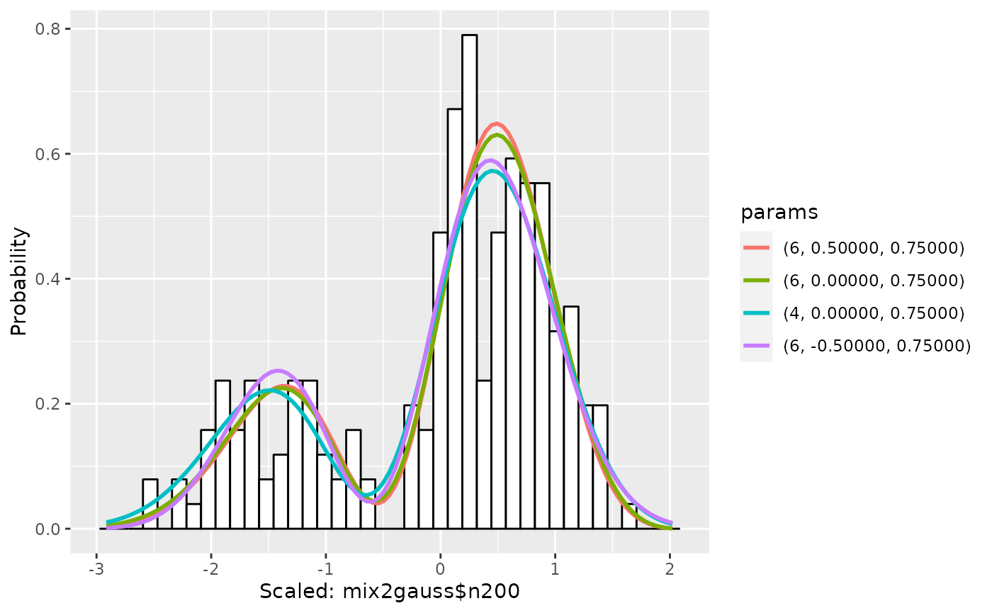

Similarly, in the legend, the color of graphs are displayed in increasing order of AIC. For example, in this graph, the estimation with the degree 6, mean 0.5, standard deviation 0.75 is the best one.

Refine estimation

We continue to estimate further by adding the degree 8 and refining mulist=seq(0, 0.5, by=0.1) and sdlist=seq(0.6, 0.9, by=0.1). Here seq command generates the vector starting from 0, incrementing by 0.1, and ending with 0.5, in case of seq(0, 0.5, by=0.1).

## Do estimation
## Output messages are suppressed for brevity
gm1 <- estimate(gm1, c(4, 6, 8), seq(0, 0.5, by=0.1), seq(0.5, 1, by=0.1),
        scaling=TRUE)

Note that parameters already estimated are skipped in estimate.gaussmodel and we omit argument names.

The summary of estimation is displayed:

## Show the summary of results up to 5
summary(gm1, nmax=5, estonly=TRUE)

##   ESTIMATION
## Name: mix2gauss$n200 
##   deg       mu1      sig1  mu sig      aic     accuracy
## 1   8 0.4503117 0.5111988 0.0 0.5 148.0353 7.618550e-08
## 2   4 0.5525515 0.7156783 0.1 0.7 148.3883 5.332699e-08
## 3   4 0.4503117 0.7156783 0.0 0.7 148.9077 5.384915e-08
## 4   4 0.6547913 0.7156783 0.2 0.7 149.4495 5.285857e-08
## 5   8 0.4503117 0.6134385 0.0 0.6 149.5980 6.356240e-08

The graphs are displayed:

plot(gm1)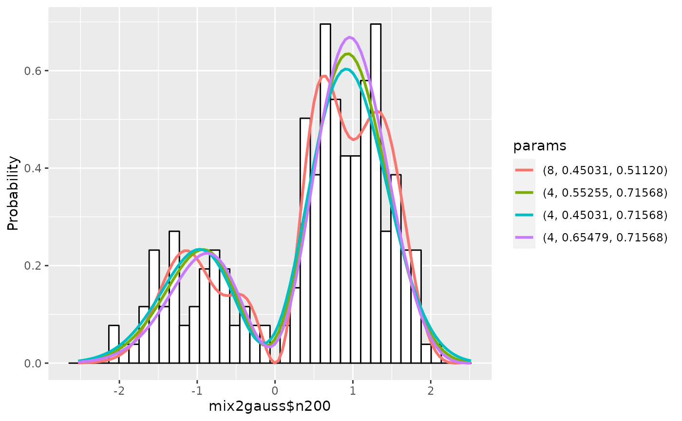

We continue to do estimation by refining parameters and checking estimates and graphs.

## Do estimation
## Output messages are suppressed for brevity
gm1 <- estimate(gm1, c(4, 6, 8), seq(0, 0.2, by=0.05), seq(0.6, 0.8, by=0.05),
          scaling=TRUE)

## Show the summary of results up to 5
summary(gm1, nmax=5, estonly=TRUE)

##   ESTIMATION
## Name: mix2gauss$n200 
##   deg       mu1      sig1   mu  sig      aic     accuracy
## 1   8 0.4503117 0.5111988 0.00 0.50 148.0353 7.618550e-08
## 2   4 0.5525515 0.7156783 0.10 0.70 148.3883 5.332699e-08
## 3   4 0.6547913 0.7667982 0.20 0.75 148.4273 5.429469e-08
## 4   4 0.5014316 0.7156783 0.05 0.70 148.5121 5.360879e-08
## 5   4 0.6036714 0.7667982 0.15 0.75 148.5294 5.448186e-08

plot(gm1)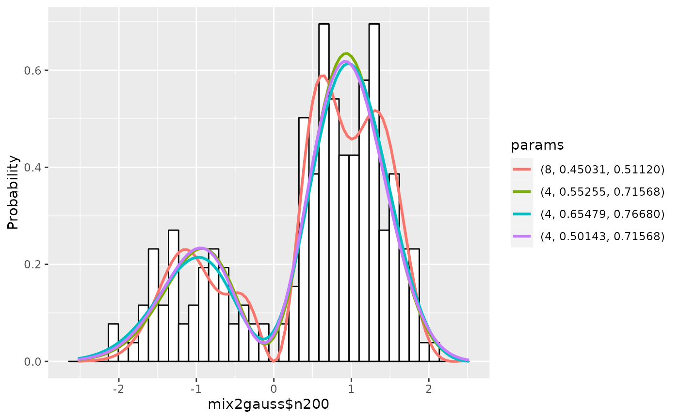

According to above results, we confine the degrees of polynomials only to 4, and set mulist=seq(0, 0.2, by=0.025) and sdlist=seq(0.7, 0.8, by=0.01).

## Do estimation
## Output messages are suppressed for brevity
gm1 <- estimate(gm1, c(4, 6, 8), seq(0, 0.2, by=0.025), seq(0.7, 0.8, by=0.01),
          scaling=TRUE)

## Show the summary of results up to 5
summary(gm1, nmax=5, estonly=TRUE)

##   ESTIMATION
## Name: mix2gauss$n200 
##   deg       mu1      sig1    mu  sig      aic     accuracy
## 1   8 0.4503117 0.5111988 0.000 0.50 148.0353 7.618550e-08
## 2   4 0.6036714 0.7463502 0.150 0.73 148.1563 5.402243e-08
## 3   4 0.5781114 0.7361262 0.125 0.72 148.1631 5.390074e-08
## 4   4 0.6036714 0.7361262 0.150 0.72 148.1694 5.373495e-08
## 5   4 0.6292313 0.7463502 0.175 0.73 148.1959 5.394311e-08

plot(gm1)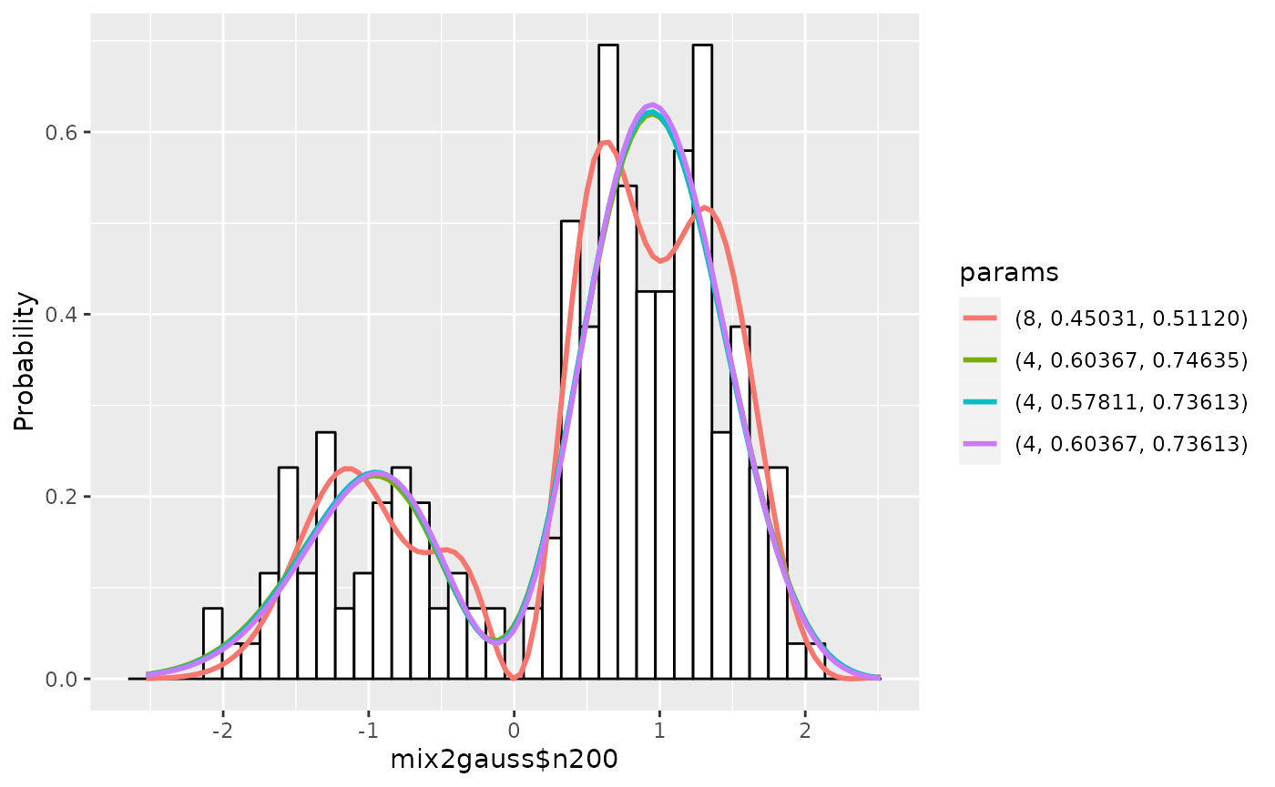

We stop doing estimation here.

Notes

Using plot.gaussmodel, we can plot cumulative distributions by setting cum=TRUE:

plot(gm1, cum=TRUE)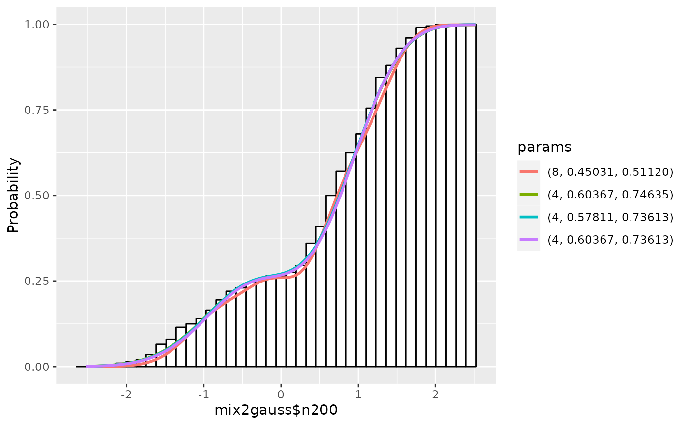

For more details, see ?plot.gaussmodel.

func.gaussmodel computes the values of density and cumulative distribution of desired estimate. For example,

x <- seq(-4, 4, by=0.1)
## Compute the density of 1st estimate
y_pdf <- func(gm1, x, n=1)
## Compute the cumulative distribution of 1st estimate
y_cdf <- func(gm1, x, cdf=TRUE, n=1)

Of course, we can compute the desired estimate by designating n=k for kth estimate shown in summary.gaussmodel.

Exponential-based Model

The density function of Exponential-based model is \[ p(x; \boldsymbol{\alpha}) \cdot \mathrm{Exp}(x; \lambda), \] where \(p(x; \boldsymbol{\alpha})\) is a polynomial with a coefficient vector \(\boldsymbol{\alpha}\), and \(\mathrm{Exp}(x; \lambda)\) is an exponential distribution with rate parameter \(\lambda\): \[ \mathrm{Exp}(x;\lambda) := \lambda e^{-\lambda x}, \quad x \in S = [0, \infty). \]

The aim of estimation is to find a good set of parameters: \(\boldsymbol{\alpha}\), \(\lambda\). To this end, we first provide a coarse set of parameters of base functions, namely, \(\lambda\), and a degree of polynomials, and then compute the coefficients of polynomials \(\boldsymbol{\alpha}\), to get a rough idea of the model.

A Creation of a model

The creation of Exponential-based model from a data set is same as that of Gaussian-based model. We will show the two scenarios, one is to create a model from only a data set, and the other is to create a model from a data set and its corresponding frequency data, in sequel.

In the first case, we use a data set mixexpgamma$n200, which contains 200 realizations of mixture of an exponential distribution and a gamma distribution, to create R’s S3 class expmodel object em1.

em1 <- expmodel(mixexpgamma$n200)

The object em1 of a S3 class expmodel contains the data and parameters to be estimated.

Similarly, in the second case, we use mixExpGammaHist$n800p for data points and mixExpGammaHist$n800f for their corresponding frequencies, to create expmodel object em2.

em2 <- expmodel(mixExpGammaHist$n800p, mixExpGammaHist$n800f)

Exploring of a data set

A summary of em1 is displayed:

## Display the summary of a data set
summary(em1)

##   SUMMARY
## Name: mixexpgamma$n200 
## The number of Data:  200 
## Mean   Std.
## 3.297944 2.491842 
## Quantile:
##           0%          25%          50%          75%         100% 
##  0.007558929  1.395016398  3.076594706  4.588611178 11.529857185 
## Quantile of Scaled Data:
##          0%         25%         50%         75%        100% 
## 0.002292013 0.422995795 0.932882670 1.391355136 3.496074388

As a name suggests, summary.expmodel shows the basic statistics of a data set. It prints out the quantiles of scaled data as well as original data. Here the scaling is to divide the data by the mean of the data.

The histogram of the data is displayed:

## Draw a histogram of the data set
plot(em1)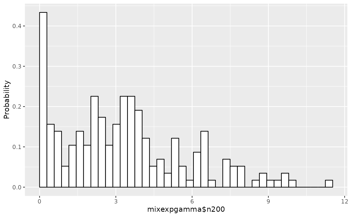

plot.expmodel can plot scaled data as well as original data by setting scaling=TRUE.

Providing the set of parameters

Before estimation, we need to provide a set of rate parameters, and degrees of polynomials, to compute the coefficients of polynomials.

## A vector of degrees of polynomials
deglist <- c(2, 3, 4)
## A vector of rate parameters of exponential distributions
lmdlist <- c(0.5, 1, 2, 4)

deglist is a vector of degrees of polynomials, in this case 2, 3, 4. In Exponential-based model, a positive integer up to around 20 is okay. Note that large degrees can cause numerical difficulty. lmdlist is a vector of means of exponential distributions, so the element of lmdlist should be positive.

Also note that the rate parameters to be passed to an estimate.expmodel method are applied to internally scaled data, not original data.

Estimation

Providing these parameter sets, we are now ready to estimate the model.

## Do estimation
## Output messages are suppressed for brevity
em1 <- estimate(em1, deglist=deglist, lmdlist=lmdlist)

The computation of the coefficients of the polynomials is done for all of the combinations of the parameter sets deglist, lmdlist, 12 cases in this example. The result is sorted according to Akaike information criterion(AIC)

Let’s see the result of estimation.

## Show the summary of results up to 5
summary(em1, nmax=5, estonly=TRUE)

##   ESTIMATION
## Name: mixexpgamma$n200 
##   deg lmd      aic     accuracy
## 1   4   2 185.4038 9.552443e-08
## 2   4   4 185.4254 9.152939e-08
## 3   3   4 191.2761 7.245070e-08
## 4   2   2 192.7590 5.681183e-08
## 5   3   2 193.7590 7.548828e-08

(nmax=5 limits top 5 estimates, and estonly=TRUE suppresses the basic statistics.)

Next see the histogram.

plot(em1)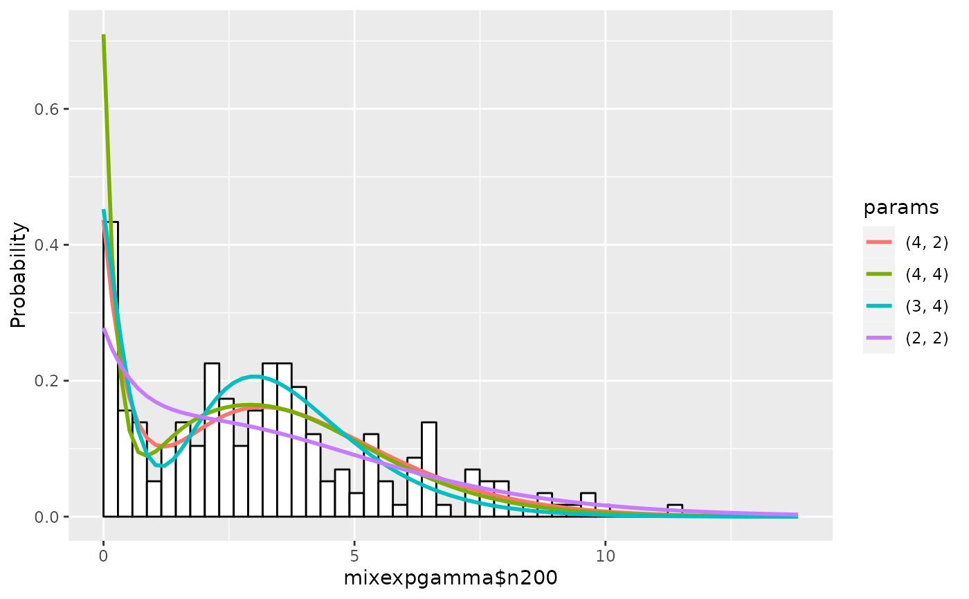

Refine estimation

We continue to estimate further by adding parameters. As we see in estimate.gaussmodel, paramters already estimated are skipped.

## Do estimation
## Output messages are suppressed for brevity
em1 <- estimate(em1, c(3, 4, 5, 6), c(1, 2, 4, 8))

The summary of the estimation is:

## Show the summary of results up to 5
summary(em1, nmax=5, estonly=TRUE)

##   ESTIMATION
## Name: mixexpgamma$n200 
##   deg lmd      aic     accuracy
## 1   5   4 183.0460 6.715527e-08
## 2   6   4 183.9109 9.767673e-08
## 3   6   2 184.7760 6.458883e-08
## 4   4   2 185.4038 9.552443e-08
## 5   4   4 185.4254 9.152939e-08

The graphs are:

plot(em1)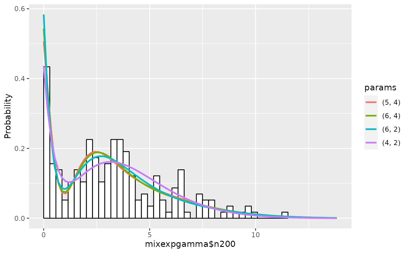

We further confine parameters as follows:

## Do estimation
## Output messages are suppressed for brevity
em1 <- estimate(em1, c(5, 6), seq(3, 4, by=0.25))

And see the summary of estimation:

## Show the summary of results up to 5
summary(em1, nmax=5, estonly=TRUE)

##   ESTIMATION
## Name: mixexpgamma$n200 
##   deg  lmd      aic     accuracy
## 1   5 3.75 183.0320 6.051334e-08
## 2   5 4.00 183.0460 6.715527e-08
## 3   5 3.50 183.4025 6.287444e-08
## 4   5 3.25 183.7779 5.609403e-08
## 5   5 3.00 183.9076 5.846981e-08

The graphs are as follows:

plot(em1)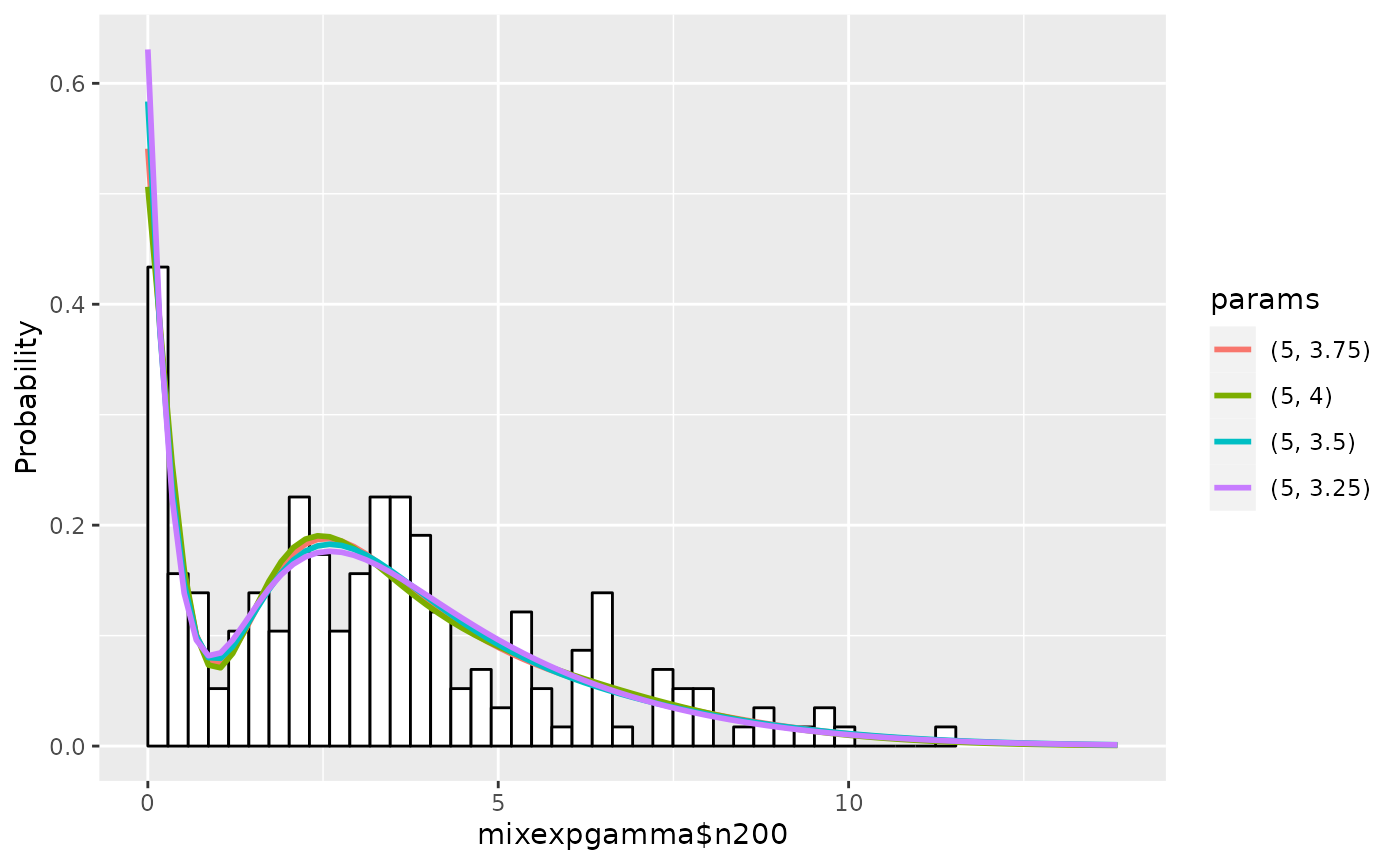

Theoretically, we can refine estimation as you like, but we stop estimation here.

Notes

Using plot.expmodel, we can plot cumulative distributions by setting cum=TRUE:

plot(em1, cum=TRUE)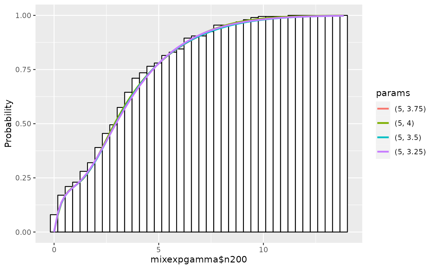

For more details, see ?plot.expmodel.

func.expmodel computes the values of density and cumulative distribution of desired estimate. For example,

x <- seq(0, 14, by=0.1)
## Compute the density of 1st estimate
y_pdf <- func(em1, x, n=1)
## Compute the cumulative distribution of 1st estimate
y_cdf <- func(em1, x, cdf=TRUE, n=1)

Of course, we can compute the desired estimate by designating n=k for kth estimate shown in summary.expmodel.